In this paper, ANSYS display dynamic analysis module LS-DYNA and flow field analysis module FLUENT are used to simulate the underwater-shell structure motion and its fluid-solid coupling phenomenon. The interface pressure data calculated by the flow field is applied to the surface of the structure in the form of loads, which cause displacement and deformation. At the same time, the structural changes further affect the distribution of the flow field. Through the reciprocating two-way coupling iteration, the dynamic response of the plate-shell structure and the distribution of the flow field are obtained. The comparison between the simulation results and the experimental results shows that this method is suitable for solving the flow-solid coupling problem with large displacement and large deformation characteristics.
1 Introduction
In nature, fluid-solid coupling phenomena are widely found in the fields of aviation, aerospace, automotive, water conservancy, petroleum, chemical, marine, and biological. In many practical problems, the influence of fluid load on the structure cannot be neglected; at the same time, the displacement and deformation of the structure will also have an important influence on the distribution of the flow field. For example, various underwater sports organizations need to consider this phenomenon.
The shell is the basic structural unit, and the simulation method of studying the process of interacting with the fluid has certain guiding significance for the design of the underwater structure. In this paper, ANSYS/LS-DYNA is used to simulate and analyze the dynamic response of plate-shell structure under underwater explosion impact load. The literature studies the flow-solid coupling problem caused by flow-induced vibration of flexible veneer in narrow flow channel. Numerical simulations, but the analysis carried out in the above literature is the vibration coupling analysis near the equilibrium position of the plate-shell structure under restraint. There are many examples of fluid-solid coupling analysis of plate-shell structures with fixed constraints using ANSYS static analysis module and fluid analysis modules such as CFX or FLUENT. ANSYS Workbench also has coupling examples in this respect. However, the dynamic analysis of the large displacement and large deformation of the structure caused by fluid shock is still not perfect, and further research is needed. Therefore, this paper applies the display dynamic analysis module LS-DYNA and the fluid analysis module FLUENT in the large-scale general finite element analysis software ANSYS13.0 to the fluid-solid coupling of the plate-shell structure with large displacement and large deformation under the impact of fluid. The effect was simulated.
2 finite element analysis
2.1 Description of the problem
In this paper, the dynamic response of the plate-shell structure under the action of fluid impact load is analyzed. The motion time history, stress distribution law and the influence on the flow field distribution of the plate-shell structure are mainly studied.
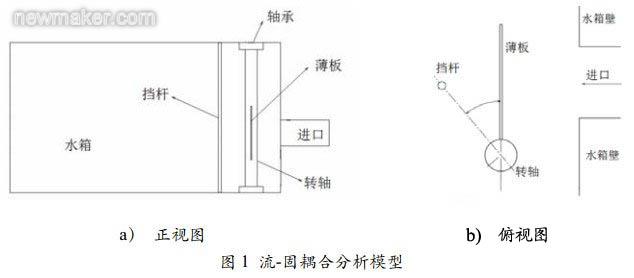
The test scheme used for the simulation comparison is shown in Fig. 1. One end of the rectangular thin plate is fixed on the rotating shaft and completely immersed in the water tank, and a high-speed water inlet is provided on the water tank wall facing the center of the thin plate to ensure the water flow at the initial stage. At the moment, the center of the sheet can be vertically impacted. In addition, a rigid baffle parallel to the center line of the rotating shaft is disposed at a specific position in the rotating direction of the thin plate in the water tank, and is intended to reverse the obstruction of the thin plate which is rotated by the impact of the fluid, so that it appears larger Deformation. The measured angle of rotation of the thin plate and the stress distribution of the plate surface can be used as the basis for the simulation comparison.
2.2 Calculation model
2.2.1 Structural model
The structural model consists of four parts: a rectangular thin plate, a rotating shaft, a bearing, and a rigid bar. The structural model can be quickly obtained by using the parametric modeling function of the ANSYS program. Using the complex solid cutting and Boolean operation functions, the structural model is all hexahedral meshed by the sweep method. The selected unit type is explicit solid164 unit, and the finite element mesh model is shown in Fig. 2.

Finite element mesh model
In addition, since it is necessary to accept the pressure load from the fluid domain calculation, and the pressure load is applied on the body unit, it is difficult to ensure the correctness of the loading. Therefore, it is necessary to establish a virtual thin shell unit on the surface of the thin plate. In the calculation process, only the pressure load is transmitted, and the thin plate structure should not be reinforced any more. Therefore, it is necessary to ensure that the thickness value of the shell unit is much smaller than the thickness of the thin plate to minimize the shell unit during the calculation. The impact on the actual calculation model. The shell element used in this paper is an explicit shell 163 unit with a solid thickness constant set to 1e-6.
The connection between the rectangular thin plate and the rotating shaft is processed by a common node. The shaft is in contact with the two bearings and the contact type is Automatic Surface To Surface. Since the thin plate will collide with the rigid bar during the rotation, contact is also required between the surface shell unit of the thin plate and the bar, and the type is Automatic Node To Surface. The total number of elements in the finite element model is 3434 and the total number of nodes is 3763.
The material of the thin plate and the rotating shaft is steel. Since the stress and deformation of the bearing are not considered, the bearing and the rigid bar are all made of a rigid material model unique to LS-DYNA and constrain all degrees of freedom.
Since the pressure load can only be applied to the part or component in the LS-DYNA, each shell element on the aforementioned divided coupling interface is established as a component, and the pressure load on each shell unit is four by the unit. The pressure values ​​of the nodes are averaged, and the pressure values ​​of the various structural nodes are interpolated from the fluid node pressure values ​​of the fluid domain according to their coordinate correspondences. After obtaining the average pressure of each unit, an array of loads is respectively established, and the load application of each unit can be conveniently performed by the APDL language.
2.2.2 Fluid domain model
The fluid domain model is modeled using the FLUENT dedicated preprocessor GAMBIT. The water tank has a length and width of 900mm, a water tank height of 500mm, an inlet pipe diameter of 90mm, and an inlet pipe length of 200mm. Because the fluid domain model is more complicated, the minimum side length of the model differs greatly from the maximum side length. Therefore, the tetrahedral unstructured grid is used for division. The division result is shown in Fig. 3. In the vicinity of the thin plate and the water inlet area, the grid density is set larger, and the grid density is set smaller at the tank wall away from the thin plate. The total number of the divided fluid domain grid is 140369. The flow field boundary conditions in FLUENT are set as follows: the inlet boundary is the velocity inlet v=5m/s, the outlet boundary is the pressure outlet p=0, and the tank wall, the rotating shaft, the thin plate and the inlet pipe wall are all wall boundaries. In addition, the wall boundary of the thin plate should be set separately to output the pressure data on the coupling surface after the fluid domain calculation is completed, and then applied to the structure solver in an externally loaded form.
2.3 Coupling method
This fluid-solid coupling problem is a two-way coupling problem, so the information transfer between the fluid and the structure is interactive. Since the result data cannot be directly exchanged between LS-DYNA and FLUENT, an intermediate data exchange step is required. In this paper, the self-programmed data conversion program is used to process the result data of the respective software calculations and convert them into data formats that can be read by the respective software, so as to perform coupling iteration. The flow of the coupling calculation is shown in Figure 4. Starting from FLUENT, the flow field is initialized first and the initial pressure distribution is obtained. Then the pressure load is transferred to LS-DYNA through data processing, and then the first time step iterative calculation of the structure field is performed. The calculated displacement data is then passed back to FLUENT through data processing to complete a coupling iteration step.
3 Simulation results analysis
3.1 Analysis of the time history of thin plate movement
Structural explicit dynamics calculations were performed using the LS-DYNA solver in ANSYS. The thin plate rotates around the rotating shaft under the action of water flow. In the ANSYS time history post-processing, the data of the centroid displacement value of the rotating plate is extracted with time, and processed into a rotation curve and an angular curve of the angular velocity with time, respectively. 5 and Figure 6. The corner and angular velocity curves measured at the same time are also given in Figures 5 and 6.
Thin plate corner time history curve
Thin plate angular velocity time history curve
By comparing the experimental and simulation curves, it can be seen that the kinematic response of the simulated thin plate using the fluid-solid coupling calculation method in this paper basically conforms to the test results. In the initial stage of the motion, since the experimental water flow rate rises from zero to a stable flow rate value, and the simulated initial flow rate is set to a stable flow rate value, the simulated corner curve slightly exceeds the test value. The maximum rotation angle of the test is slightly lower than the maximum angle of the simulation, and the collision time point of the test is ahead of the simulated collision time point. The common reason is that the surface of the test sheet is covered with a test wire, and the effect is equivalent to an increase in the thickness of the plate, so that the time point of collision with the bar is advanced, and the maximum value of the corner is lowered. It can be seen from the simulation curves of the above two figures that the duration of the entire coupling process is very short, and the time at which the thin plate finally stabilizes is about 72 ms. It can be seen from Fig. 7 that the angular velocity of the rotating plate is rapidly increased when initially subjected to fluid impact, because at the initial moment, the water flow vertically impacts the thin plate, and the thin plate receives the greatest normal force. When the angular velocity reaches a certain value, it tends to be stable, and the fluid impact load of the thin plate is balanced with the resistance of the water body and the friction torque of the rotating shaft. When t≈56ms, the thin plate collides with the rigid bar, and then a certain rebound occurs, and the angular velocity rapidly drops to a negative value. Under the continuous impact of the fluid, the amplitude of the sheet angular velocity oscillation gradually decays and tends to zero.
3.2 Thin plate stress analysis
The stress distribution of the rotating plate at different times before the collision can be obtained by using ANSYS general post-processing, as shown in Fig. 7. Because the central region of the thin plate is subjected to the instantaneous impact of the fluid, which causes the rotating shaft to rotate against the frictional resistance of the bearing and the damping of the fluid around the thin plate, the peak stress appears at the root position and decreases along the radial direction of the rotating shaft, which is a cantilever in the material mechanics. The beam bending principle is consistent. The peak stress during the rotation is maintained at around 12 MPa.
Thin plate stress cloud at different times before collision
After the thin plate rotates over a certain angle, it collides with the rigid bar. The stress distribution cloud on the collision plate is shown in Fig. 8. It can be seen from Fig. 8 and Fig. 7 that the stress distribution and stress peaks on the plate occur. Large changes, the stress peak region appears at the root and the collision contact position at the same time, and the stress peak at the root reaches 70 MPa, and the stress peak at the collision contact position also reaches 40 MPa. Since the peak value of the stress is significantly higher than the peak before the collision, the thin plate has a relatively large deformation phenomenon.
3.3 Flow field analysis
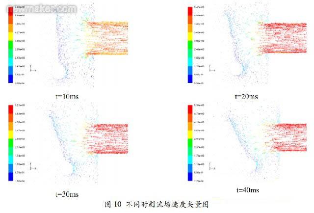
Due to the rotation of the thin plate, the flow field boundary changes at different times. Figure 9 shows the pressure field distribution in the vicinity of the thin plate at different times. It can be seen from Fig. 9 that at t=10 ms, since the expansion angle of the thin plate is small, the obstruction effect on the inlet water flow is most obvious, so that it can be seen that the entire region from the inlet to the thin plate exhibits a high pressure tendency. As time increases, the expansion angle of the thin plate becomes larger, the inlet water flow is weakened by the thin plate, and the peak pressure of the inlet region gradually decreases. Since the sheet always obstructs the inlet water flow, the maximum pressure zone remains substantially in the central region of the sheet surface and decreases toward the edge. In addition, it can be seen that as time passes, a negative pressure zone is gradually formed at the corner where the inlet meets the pipe wall, and the range of the negative pressure zone gradually becomes larger. The reason is that there is a velocity vortex here, and the time is about a long time, and the speed vortex is more obvious. The formation of the velocity vortex can be clearly seen by FIG.
Flow field pressure map at different times
4 Conclusion
The coupling analysis of the plate-shell structure with fixed constrained ends can be easily carried out by using the fluid-solid coupling module in ANSYS Workbench. However, when the structure has large rigid displacement and large deformation under the impact of fluid load, the ANSYS static implicit analysis method is not suitable for such cases. The display dynamic analysis module LS-DYNA can be used instead. Accurately simulate the kinematics of the structure and the stress distribution. In this paper, the large-scale general finite element analysis software ANSYS display dynamic analysis module LS-DYNA and fluid analysis module FLUENT complete the fluid-solid coupling simulation analysis of large displacement and large deformation caused by fluid impact. The comparison between the simulation results and the experimental results shows that for this type of fluid-solid coupling problem, the dynamic analysis module can accurately simulate the kinematics and dynamic response of the structure.

Concerned about surprises
Tag: Coupling problem Coupling Coupling calculation FLUENT LS-DYNA
Previous: Dialectical Relationships in the Field of Precision Measuring Instruments Next: Balancing the Energy Efficiency and Statics of New Synthetic Filter Media
Shower Panel,Rain Shower,Rainfall Shower
Automatic Faucet Shower Series Co., Ltd. , http://www.sinyo-faucet.com